Authors:
(1) P Aditya Sreekar, Amazon and these authors contributed equally to this work {sreekarp@amazon.com};
(2) Sahil Verm, Amazon and these authors contributed equally to this work {vrsahil@amazon.com;}
(3) Varun Madhavan, Indian Institute of Technology, Kharagpur. Work done during internship at Amazon {varunmadhavan@iitkgp.ac.in};
(4) Abhishek Persad, Amazon {persadap@amazon.com}.
Table of Links
- Abstract and Introduction
- Related Works
- Methodology
- Experiment
- Conclusion and Future Work
- References
4. Experiments
In this section, the performance of the RCT is demonstrated on a dataset of packages shipped in 2022. The mean absolute error (MAE) between the predicted and actual shipping cost is selected as the performance metric, as it is representative of the absolute error in monetary terms. In this paper, the MAE values are normalized by the MAE of day 0 heuristic estimate, which is expressed as MAE percentage (MAE%). This metric emphasizes the improvement achieved against the heuristic baseline.

4.1. Experimental Setup
4.1.1. Architecture and Hyperameters
The embedding dimension was set to 128, and 6 transformer encoder layers were used, each with 16 self-attention heads. Adam optimizer (Kingma and Ba, 2014) with a starting learning rate of 0.0001 and a batch size of 2048 was used. To improve convergence, the learning rate was reduced by a factor of 0.7 every time the validation metric plateaued. The model code was implemented using the PyTorch (Prokhorenkova et al., 2018) and PyTorch Lightning (Falcon and The PyTorch Lightning team, 2019) frameworks.
4.1.2. Data Preparation
A training dataset of 10M packages was sampled from packages shipped during a 45-day period in 2022. The data was preprocessed by label encoding categorical features and standardizing numerical features. The test dataset contains all packages (without sampling) that were shipped during a separate, non-overlapping week from 2022.
4.1.3. Benchmark Methods
We compare the performance of RCT against various models with increasing level of complexity: GBDT, AWS AutoGluon (Erickson et al., 2020), Feedforward neural network, TabTransformer and FT-Transformer. For GBDT model, numerical features were not standardized, and target encoding (Micci-Barreca, 2001) was used to encode categorical features instead of label encoding. AWS AutoGluon was configured to learn an ensemble of LightGBM (Ke et al., 2017) models. A feedforward neural network containing 5 layers was used, the input to which was generated by embedding and concatenating dimension, route and service features. Publicly available implementations [1] of TabTransformer and FT-Transformer were used, and all hyperparameters were made consistent with RCT. Since the baselines do not handle collections of items and charges, we only used dimension, route and service features.


4.2. Baseline Comparisons
Table 1a compares RCT against the baseline models discussed in section 4.1.3. The models in the table are organized in increasing order of model complexity. Both tree based models, GBDT and AutoGluon, are performing at a similar level. Deep learning models consistently outperform tree based models, indicating that the proposed architecture is efficient for shipping cost prediction. Transformer based models have lower MAE% scores than feedforward neural network, showing that transformers learn effective interaction. The RCT model outperforms both transformer models - TabTransformer and FT-Transformer (SOTA), suggesting that a custom architecture which encodes the latent structure of the rate card is contributing to the improved performance. Table 2 compares the performance of FT-Transformer and RCT models at different model sizes. The results show that RCT outperforms FT-Transformer across all tested model sizes, showing indicates that encoding rate card structure provides performance benefits across varying model capacities.
4.3. Does RCT learn effective representation of rate cards?
Transformers have been shown to have strong representation learning capabilities in a variety of tasks. In this experiment, we investigate the effectiveness of rate card representation learned by RCT. To evaluate this, we compare the performance of our GBT model with and without the learned rate card representation as an input feature.

The pooled output of the final Transformer layer is treated as the learned representation of the rate card. Adding this feature improved the performance of the GBDT by 9.79% (refer Table 1b). Further, it was observed that even when all manually engineered features are dropped, the GBDT still performs comparably, with an MAE percentage of 69.21%. This indicates that the learned representations of rate cards are not only effective at capturing better feature information, but are also sufficient representation of the package rate card. However, even with this feature, the GBDT has a 13.5% higher MAE% than the RCT. This is likely because the RCT is trained end-to-end, while the GBDT uses features learned as part of a separate model.
4.4. Does self-attention learn better interactions than feed forward neural networks?
In section 4.2, it was observed that feed forward (FF) neural networks were outperformed by transformers, leading to the hypothesis that self-attention is a superior interaction learner. This section aims to explore this hypothesis further by utilizing FF instead of self-attention to encode dimension, route and service features while limiting the width of self-attention to only the item and charge features. The output encodings of both FF and self-attention are concatenated and fed into an FF layer to predict shipping cost. As the self-attention width is decreased, it fails to capture the interactions between all rate card features. The resulting model exhibits a higher MAE% of 64.73% in comparison to the RCT’s 55.72%. These results suggest that FF models are inferior interaction learners in comparison to transformers.
4.5. Analysis of Self-Attention
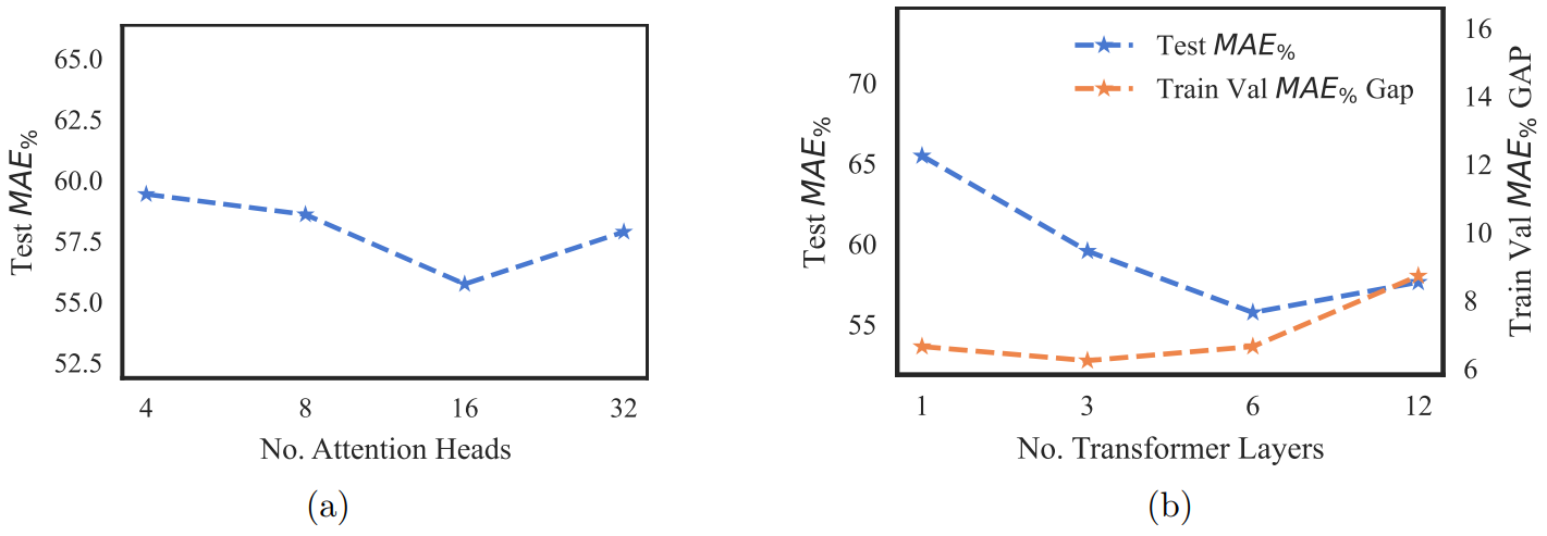
In section 3.2, we discussed the proficiency of transformers in feature aggregation, owing to self-attention. In this section, ablation experiments are conducted to analyze the effect of attention depth and attention head count. Increasing the number of attention heads allows the model to learn more independent feature interactions. For this experiment, the


model capacity is fixed at 128 dimensions, so an increase in the number of heads also reduces the complexity of interactions learned per head. Thus, choosing optimal head count is a trade-off between learning independent interactions and the complexity of each learned interaction. The trade-off can be observed in Fig. 2a, where the performance improves from 4 heads to 16 heads because the attention learned by each head is complex enough. However, the performance degrades when attention heads are increased from 16 to 32 because the complexity of heads has reduced substantially, negating the benefit of learning more independent interactions.
Next, we illustrate the effect of increasing the attention depth by adding transformer encoder layers. Deeper transformer networks learn more complex higher-order interactions, thereby enhancing the model’s performance, as observed in Fig. 2b. However, increasing the number of layers from 6 to 12 reduces the model’s performance due to overfitting, caused by the rise in learnable parameter count. The evidence for overfitting can be found in Fig. 2b, where the gap between train and val MAE increases by 30% when moving from 6 to 12 layers.

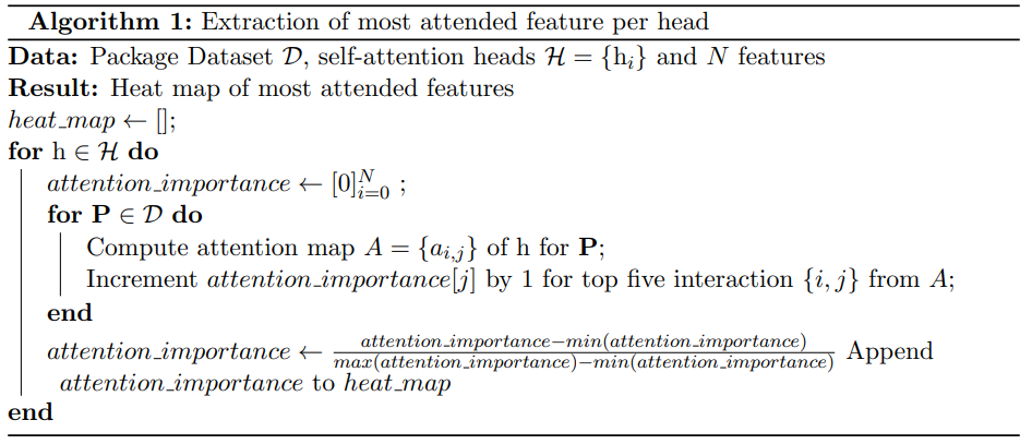
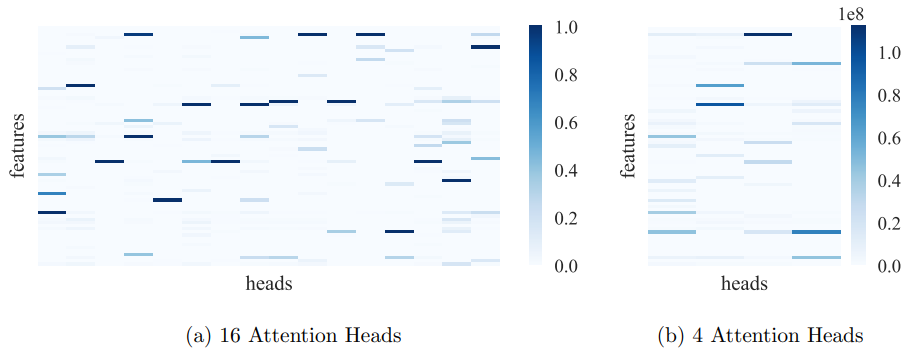
Finally, in Fig. 3, we display the heat maps generated using Algorithm 1. These heat maps illustrate the number of times each feature was attended to as part of the top five most attended features. Each column corresponds to a head, and each row corresponds to a feature. The heat map on the left was generated using RCT with nheads = 16, and the one on the right was generated with nheads = 4. Comparing both the heat maps, it can be seen that Fig. 3a has less number of active feature interactions per column, confirming our hypothesis that a larger number of attention heads leads to each head learning independent interactions between features.
4.6. How does the Transformer scale with more data?
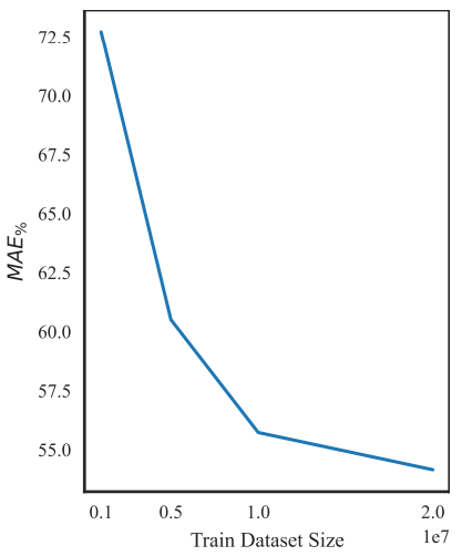
To minimize the experimentation costs, all experiments in this paper were conducted using a training dataset of size 10 million. However, it is important to use the best performing model, the training dataset size can be increased to achieve optimal performance.
To verify the scalability of RCT with data, we trained the model on different training dataset sizes and plotted the results in Fig. 4. The results demonstrate that RCT’s performance continues to improve with larger datasets. Therefore, we can confidently expect that models trained on larger datasets will outperform the model explored in this paper.
This paper is available on arxiv under CC BY-NC-ND 4.0 DEED license.
[1] https://github.com/lucidrains/tab-transformer-pytorc

